3. Input-Output-models | 1999-06-28 To Chap 2 |
General equilibrium models consist of a input-output model and assumptions about how the volume of the consumption depends upon the prices. The prices are in turn calculated from the costs of the primary production factors, labor and capital. The cost of labor is determined by the wage level. The profits of the enterprises are regarded as part of the capital costs.
"A general equilibrium model considers the economy as a system of mutually interdependent markets. A change that at a first glance only affects one market, can in practice affect all markets of the economy ". … "Similar models are now used by the World Bank and other organizations for the evaluation of economic policies ". Cited for the final report of the Swedish Government Commission on Green Taxation, pages 325 and 328, ref. (1).
General equilibrium models constitute the accepted theory for analyzing economies and the impacts of political decisions. The book "Notes and Problems … ", ref. (2) calls it "Practical Policy Analysis". The book has a thorough description of the theoretical foundations. Input-output models and a bigger model called the DMR model (after the designers Dervis, Melo and Robinson) are described. It is said about the DMR model that: "Variants exist for about a dozen countries and have been used in regular reporting and advising functions of the World Bank".
Input-output models are described in chapter 3 of the book "Economic theory" ref. (3). The book also describes production processes and flow diagrams.
This chapter will describe the basic ideas and show how they can
be treated by the methods developed in chapter 2
"Basic Principles".
The book "Notes and Problems … ", ref. (2), starts in chapter 1 with a introductory example of a hypothetical society that produces only two products, wine and cloth. The author works in Australia, hence the choice of products. "The techniques currently in use for the production of these products are described by input-output coefficients in Table 3.2:1. The output of one gallon of wine requires an input of 0,2 yards of cloth and one hour of labor. The output of one yard of cloth requires an input of just one hour of labor. We assume the society's resource endowment for a year is 100 labor hours."
| Inputs | Wine | Cloth |
| Wine | nil | nil |
| Cloth | aw = 0,2 yards/gallon | nil |
| Labor | lw = 1 hour/gallon | lc = 1 hour/yard |
Table 3.2:1 Input-Output coefficients for a wine-cloth
economy.
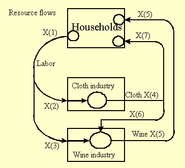
The system can be described by a circuit diagram that shows the flows of resources. The payment flows have not been treated so far.

Figure 3.2:1 Resource flows for a wine-cloth economy.
The households do not consume all cloth that is produced, some is used in the production of wine, i.e. cloth is an intermediate product in the system. The following equations can be formulated for the system:
| Flow balances | ||
| Labor supply (h) | X(1) - X(2) - X(3) = 0 | Eq 3.2:1 |
| Use of cloth (yard) | X(4) - X(6) - X(7) = 0 | Eq 3.2:2 |
| Process equations | ||
| Labor (h) -> cloth (yard) | X(2) - lc*X(4) = 0 | Eq 3.2:3 |
| Labor (h) -> Wine (gallon) | X(3) - lw*X(5) = 0 | Eq 3.2:4 |
| Cloth (yard) -> Wine (gallon) | X(6) - aw*X(5) = 0 | Eq 3.2:5 |
Table 3.2:2 Equations for wine-cloth economy.
The equations have 7 variables X(1) - X(7) and 3 parameters, labor requirement lc = 1h/yard for producing cloth (labor for cloth), labor requirement lw = 1h/gallon for producing wine (labor for wine) and the need of cloth aw = 0,2 yard/gallon in the wine production.
7 variables and 5 equations gives 7-5 = 2 degrees of freedom. Two variables can thus be determined arbitrarily. In the problem 1.1 of ref. (2), the question is how much can be produced with a given quantity of labor. We set the labor supply to Y(1) (h) and choose the consumption of wine Y(2) (gallon) as the other variable. This gives another two equations:
| Total labor supply (h) | X(1) = Y(1) | Eq 3.2:6 |
| Final consumption of wine (gallon) | X(5) = Y(2) | Eq 3.2:7 |
Table 3.2:3 Equations with exogenous variables for wine-cloth
economy.
By adding two equations, that may seem to be trivial, it will be easier to change the restrictions of the system and calculate different variations within the framework of the system. The equations 3.2:1-5 are general and need never to be changed.
The first question posed by the author is: What can be produced?
What combinations of wine and cloth quantities are possible to
produce by using a total of 100 hours of labor? Put Y(1)
= 100 h, and vary Y(2) from 0 to 100 gallons and solve
the equation system for each value of Y(2). The labor is
redistributed from producing cloth to the production of wine.
It can be expected that the quantity of cloth diminishes when
the production of wine increases. The problem is solved the appended
Excel-calculus. The result is shown
in the diagrams below:
 | 
|
| 1 hour of work per yard of cloth | 0.5 hour of work per yard of cloth |
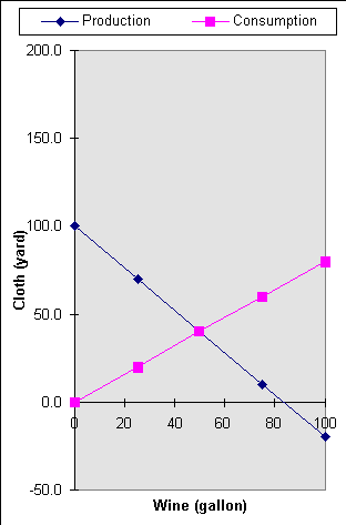
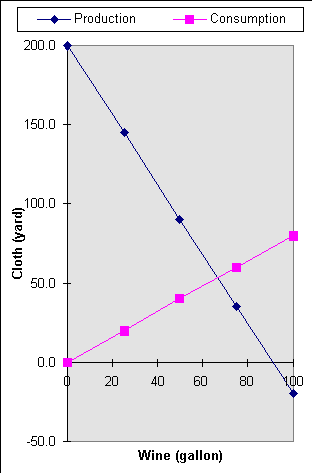
Figure 3.2:2 Final output of cloth (yard) as a function of the output of wine (gallon) with the use of 100 hours of labor (Two cases, lc = 1 and 0.5 h/yard).
The production line shows the production alternatives that are possible by different distributions of 100 hours of labor. The alternatives that require less labor are found below the line. It is not possible to produce the alternatives above the line by the use of the available amount of labor. When 100 gallons of wine are produced we get a deficit of 20 yards of cloth. It is not a possible combination, unless the stocks are reduced or cloth is imported.
Now when we have calculated the production possibilities (net output) of the society, the next question is: What will be produced? "This will depend on the level of employment and consumer preferences for wine and cloth."
Make the simple assumption that wine and cloth are consumed in fixed proportions, e.g. 5 gallons of wine and 4 yards of cloth.
| Consumer preferences (yards of cloth /gallons of wine) | -c2w*X(5) + X(7) =0 | Eq 3.2:6a |
| Final consumption of wine (gallons) | X(5) = Y(2) | Eq 3.2:7 |
Table 3.2:4 Equations for certain consumer preferences
in the cloth-wine economy.
The consumption line, figure 3.2:2, shows the volumes of the two commodities at varying consumption volume. The are consumed at the ratio c2w (cloth to wine). The consumption line intersects the production line in a point where the consumption and the production of the two goods coincide. This point can be calculated by the use of the following two equations:
| Consumer preferences (yards of cloth /gallons of wine) | -c2w*X(5) + X(7) =0 | Eq 3.2:6a |
| Total use of labor (h) | X(1) = Y(1) | Eq 3.2:6 |
Table 3.2:5 Equations for certain consumer preferences
and use of labor in the cloth-wine economy.
With c2w = 4/5 yards/gallon and Y(1) = 100 hours we get the following flows in the point of intersection:
| Labor requirement in the cloth industry, lc | 1 hour/yard | 0.5 hour/yard |
| Total amount of labor X(1) | 100 h | 100 h |
| Labor in the cloth industry X(2) | 50 h | 33 h |
| Labor in the wine industry X(3) | 50 h | 67 h |
| Produced cloth X(4) | 50 yard | 67 yard |
| Produced wine X(5) | 50 gallon | 67 gallon |
| Cloth used in the wine industry X(6) | 10 yard | 13 yard |
| Cloth delivered to the households X(7) | 40 yard | 53 yard |
Table 3.2:6 The resource flows of the system.
The left column shows the flows at the original circumstances. The households will consume 50 gallons of wine (= production of wine) and 40 yards of cloth. What happens if the productivity in the cloth industry increases, i.e. 2 yards of cloth are produced per working hour? Provided that the consumer preferences remain the same, the households will consume 67 gallons of wine and 53 yards of cloth. The production of both goods increase by the reallocation of 17 working hours from the cloth industry to the wine industry. However, there are some important preconditions:
If the hourly wages are assumed to be wc = ww = $1 and if the prices only reflect the marginal costs, then the costs and the total wages will be:
| Labor requirement in the cloth industry, lc | 1 hour/yard of cloth | 0.5 hour/yard of cloth |
| Price of cloth | pc = lc * wc = $1/yard | pc = lc * wc = $0.5/yard |
| Price of wine | pw = aw * pc + lw * ww = $1.2/gallon | pw = aw * pc + lw * ww = $1.1/gallon |
| Total wages to workers in the cloth industry | $50 | $33 |
| Total wages to workers in the wine industry | $50 | $67 |
| Total cost of cloth to consumers | $40 | $26 |
| Total cost of wine to consumers | $60 | $74 |
Table 3.2:6 Payment flows of the system.
Because the wine industry buys cloth, the cost of the product
will be greater than the cost of the labor. When the productivity
in the cloth industry increases, the payment flows are redistributed,
more money is paid for wine and both product become cheaper. In
practice, the consumption of cloth will increase more than the
consumption of wine because cloth has the biggest price reduction,
and people can afford to sew more clothes.
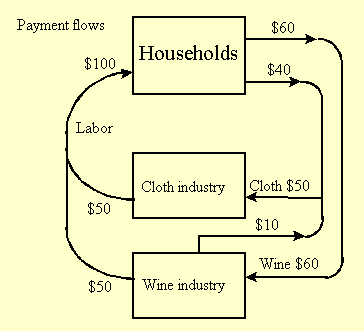
Figure 3.2:3 Payment flows for the wine-cloth economy
when the labor requirement is 1 hour/yard of cloth.
The flows can be summed up in an input-output table:
| To | Usage | |||
| From | Cloth industry | Wine industry | Private consumption | Total output |
| Cloth industry | 0 | $10 | $40 | $50 |
| Wine industry | 0 | 0 | $60 | $60 |
| Labor | $50 | $50 | ||
| Total input | $50 | $60 | ||
Table 3.2:7 Input-output table, all flows are quantified as money and flow in the opposite direction of the payment flows (labor requirement is 1 hour/yard of cloth).
This input-output model describes only the production system of
the economy. The rest of the society is not treated. The model
calculates the production in the different parts of the production
system when the demand (final usage) and/or the usage of labor
(primary production factors) are known.
(The rest of this chapter will be elaborated later.)
Back to home page, contents,
beginning of chapter.
Next chapter Chap 4.