4. Calculation example with Swedish economic system | 1999-06-28 To Chap 3. |
| Model S1 |
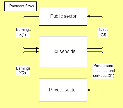
First a very simple example is shown. It is the circuit diagram of Model S1 (Static no 1).

Figure 4.1:1, Model S1
The model has four payment flows X(1) through X(4). In this simple model, all incomes from the selling of goods and services are used to pay wages and salaries. The balance of payments for the private sector is described by the equation X(1) = X(2). The flow into the private sector (the enterprises) equals the flow out from the sector. The same principle holds for other sectors, the sum of the flows into the sector equals the sum of the flows from the sector.
We get the following payment balances:
| Private sector: | X(1) = X(2) | eq. (1) |
| Households: | X(2) + X(4) = X(1) + X(3) | eq. (2) |
| Public sector: | X(3) = X(4) | eq. (3) |
Table 4.1:1
The equations also describe the connections between the sectors. The payments of the households for goods and services X(1) flow to the private sector. These money become wages and salaries X(2) that go back to the households.
It is known from the algebra that four linearly independent equations
are needed in order to calculate four unknowns. A close view on
the three equations above reveals that if equation (2) is added
with equation (1), the result is
X(1) + X(2) + X(4) = X(1) + X(2) + X(3). The terms X(1)
+ X(2) are part of both the left and the right members of
the equation and can be eliminated. That yields X(4) = X(3)
which is the same as equation (3). The three equations are linearly
dependent and that makes one equation superfluous. Equation (3)
can be omitted. For a closed system, one of the balance equations
will not be needed.
Thus, we need two additional equations in order to determine the four unknowns. These can be chosen as:
| Taxes: | X(3) = s * ( X(2) + X(4) ) | eq. (4) |
| Private production: | X(1) = priv.prod. | eq. (5) |
Table 4.1:2
Equation (4) says that one share of the total incomes of the households is paid as taxes, s is the tax rate. Equation (5) tells that the households use their whole available income (what is left when taxes have been paid) and that the size of the private production is known in some way.
The unknowns can be calculated by successive elimination from equation to equation but we will use a general method instead and formulate the problem as a system of equations.
| Private sector: | X(1) - X(2) = 0 | eq. (1´) |
| Private production: | X(1) = priv.prod. | eq. (2´) |
| Households: | -X(1) + X(2) - X(3) + X(4) = 0 | eq. (3´) |
| Taxes: | s*X(2) - X(3) + s*X(4) = 0 | eq. (4´) |
Table 4.1:3
The equations have been reordered and renumbered. First come the equation for the private sector, balance of payments and an assumption about the volume of the production. Then come two equations for the households, balance of payments and taxes. The unknown quantities X(.) are ordered according to increasing index and to the left of the equal sign. Payment flows into a sector have a plus sign, payment flows from a sector have a minus sign. The given quantity priv.prod. is placed in the right member.
The equation system can now be written in matrix form:
| M(s) = | / | 1 | -1 | 0 | 0 | \ | Y = | / | 0 | \ |
| | | 1 | 0 | 0 | 0 | | | | | priv.prod. | | | ||
| | | -1 | 1 | -1 | 1 | | | | | 0 | | | ||
| \ | 0 | s | -1 | s | / | \ | 0 | / |
Using matrix notation yields:
M(s) * X = Y
M(s) is the system matrix that determines the properties of the system. The tax rate s is the only parameter in the matrix and determines the distribution between taxes and private consumption. The private production is found in the right member Y which determines the size of the economy.
The model says nothing about the level of tax rate s or the size of the private production priv.prod. The tax rate may be called a decision quantity and the private production a quantity to be forecast (or a state variable). If these are known then the flows can be calculated.
The payment flows X are the endogenous variables of the system, the quantities s and priv.prod are the exogenous variables of the system.
The resource flows are not included in the calculations for this
simple model, but are shown in the diagram below: 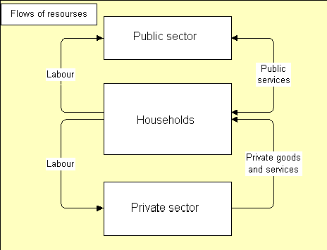
Figure 4.2:1 Resource flows for the simple economic system.
The labor comes from the households to the private and public sectors. Privately produced goods and services are delivered to the households. Public services are consumed by the members of the households but are often received at the public institutions, such as schools and hospitals, thus arrows in both directions. The total earnings are related to the volume of labor by the level of wages and salaries. The total payments for the commodities are related to the volume by the price level. There is no direct relation between the amount of taxes paid by each household and the benefit of public services. The public services are shared according to the need between households and generations.
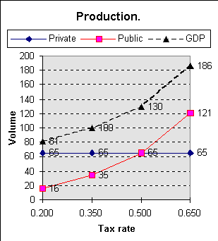
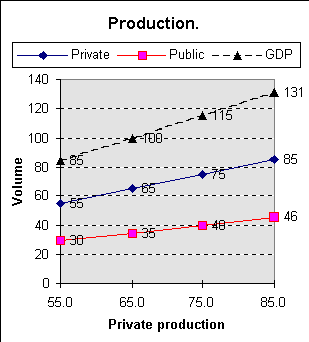
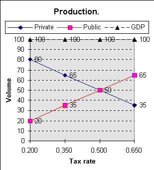
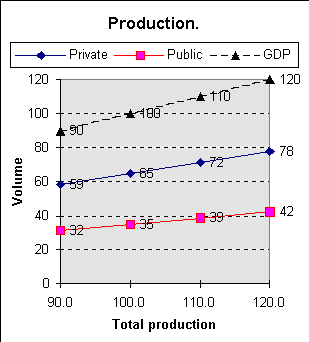
The results from two calculation examples with the previous equations are shown below. Both cases are chosen so that the second point in the diagrams have the tax rate = 0.35 and GDP = 100 (arbitrary units):
 | 
|
| Figure 4.3:1 | Figure 4.3:2 |
| Tax rate varies, Private production = 65 | Private production varies, Tax rate = 0,35 |
The diagram shows that increasing the tax rate gives more money
for the public sector. The private production does not suffer.
Fantastic! As an alternative we can wait until (or hope for that)
the private production increases. Note that the private production
is one of the given quantities of the equation system.
What happens if equation (2) is formulated with the total production
as given?
| Total production: | X(1)+X(4) = total.prod. | eq. (2´´) |
Then the same variable variation as example 1 above give this
result:
 | 
|
| Figure 4.4:1 | Figure 4.4:2 |
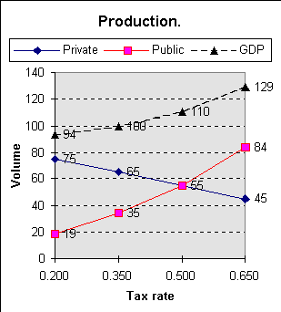
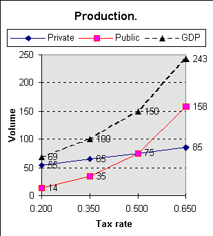
| Tax rate varies, Total production = 100 | Total production varies, Tax rate = 0,35 |
An increase of the tax rate results in a catastrophe. The private production decreases when the public production increases. An increase of the private production works in this case also.
Why so different results? The examples show clearly that it is important to choose the right equations. The equations should be chosen so that the exogenous quantities as close as possible are constant when the other parameters vary.
Example 1 can be considered as most realistic at a high rate of unemployment and no bottlenecks in the economy. At a low rate of unemployment, the total production is limited by the availability of labor and example 2 may be closer.
The contradiction between the simulation with private production given (point 4.3) and with total production given is not real. It is actually the same model with different restrictions. If the total production is increased in the latter case as the tax rate is increased (e.g. total.prod. = 186 and s = 0.65), then the two simulations will give the same result.
The diagrams above only compare different states of the economy
with one another. The model does not say if a real development
will move from one state to the other. The question about which
states will follow one another can only be answered by a dynamic
model.
In real life, there are no pure cases, tax rate and production vary at the same time. This model says nothing about the interdependence between the two or the dependence of the other flows.
 | 
|
| Figure 4.5:1 | Figure 4.5:2 |
| Private production decreases | Private production increases |
In the first case, one may assume that the private production
decreases because the private purchasing-power diminishes . In
the other case, the total demand increases and that should be
advantageous for the private production. Only studies of historical
data can show what happens in reality.
The Excel calculus used for the calculations can be downloaded
here.
Back to home page , contents, beginning of chapter.
Next chapter Chap 5 .